See also Experimental Design, Cochran and Cox, Chapter 4

The Completely Randomised Design (CRD/One-way ANOVA) is a very simple, powerful and convenient design in many cases. It is appropriate when we have 1 factor with 2 or more levels. The example given for a CRD had 1 factor (treatment) with 6 levels (the 6 treatments). Howver, we require all treatments to be carried out contemporaneously; the treatments being assigned to the experimental units randomly. Sometimes this is not possible or not completely what we want. We may have more than 1 factor that influences the response. For example, suppose that we wanted to compare 6 diets for feeding to pigs and that we have the facilities, space, resources, time, etc for 12 pigs; so that we could have 2 pigs per diet (for a simple CRD). Perhaps we have both male and female pigs and we would like to incorporate this into our model and analysis. Thus we will require a model with more than 1 factor; a 2 factor model, one factor being our 6 treatments and the other factor being the 2 sexes. We have 6 male pigs and 6 female pigs and we specifically assign 1 male and 1 female pig to each of the six diets. The 12 pigs are in individual cages (pens), randomly assigned and within each sex the assignment to diets is at random. This random assignment is our only hope of ensuring that we can consider the observations to be independent of one another. The following data were obtained:

Weight gain of pigs

Sex	Diet 1	Diet 2	Diet 3	Diet 4	Diet 5	Diet 6
Female	27.4	17.7	17.0	21.7	12.3	17.3
Male	33.6	25.8	20.4	23.0	13.4	20.8

A suitable model to describe each observation would therefore be:

Y_ij = µ + trt_i + sex_j + pen_ij + animal_ij + e_ij

as before for our CRD problem, with only 1 observation per animal and 1 animal per pen we cannot seperate pen_ij animal_ij and residual_ij effects, they are 'confounded' or combined into one error term, e_ij.

and

Thus our linear model now becomes :

Y_ij = µ + trt_i + sex_j + e_ij

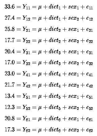
and

Thus our equations are :

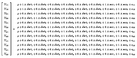
And in matrix notation (Y = Xb + e) we have

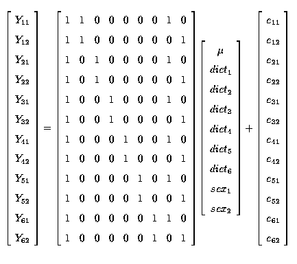
Note that if we look at the columns of X we can see that columns 2 + 3 + 4 + 5 + 6 + 7 sum to column 1 ( µ ) and that columns 8 + 9 also sum to column 1 ( µ ). This means that there are 2 linear dependencies and that therefore although X has 9 columns it only has rank of 9-2 = 7, i.e. r(X) = 7.

With a model starting with only µ (column 1) then for the 6 subsequent columns (columns 2 to 7) relating to diets (treatments) there are only 5 that are linearly independent; which means that there are only 5 degrees of freedom (d.f.) for diet. Similarly, for the columns relating to the sex effects (columns 8 and 9) there is only 1 that is linearly independent, which means that there is only 1 d.f. for sex.

What this means relates directly to our tests of hypotheses.

The hypothesis test for diets (treatments) is :

which we can re-write as :

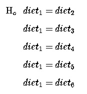
or re-writing, so that our Null Hypothesis is equal to zero, we get :

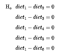
There are 5 comparisons here, which correspond to the 5 d.f. for diets; 5 linearly independent comparisons between our 6 diets.

Thus a suitable k' matrix to compute these contrasts would be

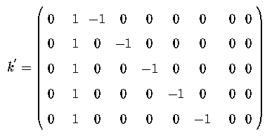
Which would translate into the following SAS contrast statement, to explicitly generate the Sums of Squares for Diets

contrast 'SS diets| mean, sex' diet 1 -1 0 0 0 0,
                               diet 1 0 -1 0 0 0,
                               diet 1 0 0 -1 0 0,
                               diet 1 0 0 0 -1 0,
                               diet 1 0 0 0 0 -1;

These are not the only possible 5 linearly independent comparisons that we could have chosen. Work out other combinations.

Similarly the hypothesis test for the sex effect is :

Which we can re-write as :

Which gives us our 1 d.f. for sex.

What are the 2 k' matrices for these comparisons/contrasts?

With these 2 k' matrices, or CONTRASTS in SAS GLM terminology, we can combine these to produce a k' matrix, and a CONTRAST, that will generate the Redusction Sums of Squares for the model over and above the mean, i.e. SSR_m:

contrast 'SSRm diets, sex| mean' diet 1 -1 0 0 0 0,
                                 diet 1 0 -1 0 0 0,
                                 diet 1 0 0 -1 0 0,
                                 diet 1 0 0 0 -1 0,
                                 diet 1 0 0 0 0 -1,
                                 sex  1 -1;

Two way ANOVA

Source of variation	d.f.	Sums of Squares	Mean Squares	F-ratio	Prob.
Total	N = 12	5626.48
Model	r(X) = 7	5607.513	801.07
C.F. mean	1	5225.013	5225.013
Model after µ	r(X)-1 = 6	382.5	63.75	16.81	.0036
Trt | µ , Sex	5	336.080	67.217	17.72	0.0034
Sex | µ , Trt	1	46.133	46.133	12.24	0.0173
Residual	N-r(X) = 5	18.966	3.7933