How can we test for, or check for, normality if we do not know whether our observations are normally distributed, or not? We need to test for skewness and kurtosis. This is easily done using SAS, with the procedure PROC UNIVARIATE. Proc Univariate provides simple descriptive statistics for numeric variables, including testing for normality. The Shapiro-Wilk statistic (W) is used for sample sizes below 200. It is important to note that it is the residuals that should be tested for normality; in this way the fixed effects components do NOT enter into the calculations and hence cause no bias.

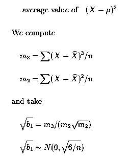
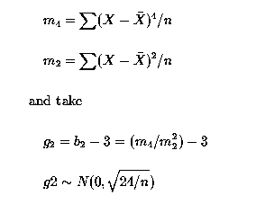
For large sample sizes the data can be tested against a normal distribution using measures of the third and fourth moments about the mean, to estimate the degree of skewness and/or kurtosis.

Let us start with a simple situation. Suppose that we have a population of cows with a mean lactation milk yield of 7500 kg.

It is the distribution of the error terms (the e's) which determines the distribution of the Y's. Whatever is the distribution of ( µ + e) will determine the distribution of the Y's, our dependent observation (conditional upon the effect of any fixed effects/independent variables in our model).

Since µ is a fixed effect and hence has no distribution it therefore follows that :

So what is the distribution of the e's (the error, or residuals)?

We use the first moment about the mean to estimate the mean ( µ ).

We use the second moment about the mean to estimate the variance.

We use the third moment about the mean to estimate the skewness.

We use the fourth moment about the mean to estimate the kurtosis.

So, if we estimate the mean as the average of the observations (Y's), we can estimate the e's as : e = (Y - E(Y)) = Y - µ

The third moment about the mean is used to measure the skewness in a population; the average value of (X - µ)³.

The fourth moment about the mean is used to test for kurtosis; the average value of (X - µ)⁴.

Consider the multiple regression problem, where we had 30 observations and 3 regression variables (X1, X2 and X3), Multiple Regression I. Our statistical model was:

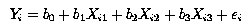
We can make use of SAS to compute the estimated residuals for each observation (this removes the fixed effects components, Xb) and then we can sensibly test these residuals for Normality, using PROC UNIVARIATE. The following code shows how we use SAS to fit the multiple regression model, output the variables (Y, X1, X2 and X3) as well as the predicted/fitted values and the residuals for each observation to a new SAS dataset (using the OUTPUT statement), which we can then use as input to PROC UNIVARIATE to test for Normality.

data reg1;
input x1 x2 x3 y;
cards;
 3.05 1.45 5.67 0.34
 4.22 1.35 4.86 0.11
 3.34 0.26 4.19 0.38
 3.77 0.23 4.42 0.68
 3.52 1.10 3.17 0.18
 3.54 0.76 2.76 0.0
 3.74 1.59 3.81 0.08
 3.78 0.39 3.23 0.11
 2.92 0.39 5.44 1.53
 3.10 0.64 6.16 0.77
 2.86 0.82 5.48 1.17
 2.78 0.64 4.62 1.01
 2.22 0.85 4.49 0.89
 2.67 0.90 5.59 1.40
 3.12 0.92 5.86 1.05
 3.03 0.97 6.60 1.15
 2.45 0.18 4.51 1.49
 4.12 0.62 5.31 0.51
 4.61 0.51 5.16 0.18
 3.94 0.45 4.45 0.34
 4.12 1.79 6.17 0.36
 2.93 0.25 3.38 0.89
 2.66 0.31 3.51 0.91
 3.17 0.20 3.08 0.92
 2.79 0.24 3.98 1.35
 2.61 0.20 3.64 1.33
 3.74 2.27 6.50 0.23
 3.13 1.48 4.28 0.26
 3.49 0.25 4.71 0.73
 2.94 2.22 4.58 0.23
;

proc glm data=reg1;  /* Using PROC GLM (General Linear Model)  */
model y = x1 x2 x3;
output out=reg2 p=yhat r=ehat;
run;
quit;  /* Exit PROC GLM  */

proc univariate data=reg2 normal;
var ehat y;
run;

If we look at the output from PROC UNIVARIATE, we see that when we test the ehat's for Normality, we obtain a Probability of 0.1135, that is to say that there is an 11% chance of obtaining such a distribution of residuals when the Null Hypothesis (that the residuals ARE Normally distributed) is true. Thus we would/should/could accept that the residuals are normally distributed, hence one of our assumptions required for our ANOVA and tests of significance is met.

If we had used the Y values and simply tested them for Normality, we would have obtained a Probability of 0.0371, i.e. we would have concluded that there was only a 3.7% chance of obtaining such a distribution of residuals when the Null Hypothesis was true. Therefore we would have ended up (erroneously) rejecting H_o and therefore accepting H_A (that the residuals were not Normally distributed)!

Reference: Snedecor and Cochran, Statistical Methods.
see: Skewness and Kurtosis. Chapter 3.13 and 3.14

Reference: Shapiro, S.S. and Wilk, M.B. An analysis of variance test for Normality (complete samples).
Biometrika, 52, P591-611.

Reference: SAS Procedures Guide, PROC UNIVARIATE, Test of Normality.