Reference : SAS System for Mixed Models
Repeated measurements are quite common in biological experimentation. One problem, if one can call it that, is that the term repeated measures means several things, depending upon the type of repeated measurement and the covariance structure.
- multiple measurements of a response variable on the same experimental unit. Often we will not simply take one measurement from each experimental unit (animal), but rather we will take several measurements, often over a period of time. An example will serve to illustrate this; suppose that we have an experiment to compare six diets for their effect on milk production in dairy cattle. We assign 5 cows to each diet and record their production throughout a complete lactation. We could add up all their individual recorded productions to have 1 value for the total milk production of each cow (commonly her 305-day milk yield). This would give us 1 measurement (of milk yield) per cow, 5 cows per treatment and 6 treatments, for a total of 30 measurements, in a simple One-way ANOVA, Completely Randomised Design. However, rather than analyse the one, 305-day milk yield value, suppose that we decide to analyse the individual daily milk yields of the cows. Now we will have several (perhaps up to 305!) records on each cow; the measurements are not independent of one another, they are repeated measurements on the same experimental unit (the cow).
examples
Dairy cows:
2 treatments, 10 cows per treatment (diet).
- measure the milk yield each day (week, month)
the cow is the experimental unit; to which the treatment/diet was applied.
daily milk yield is the response variable for which we have multiple measurements.
Growing animals:
2 diets, from weaning to slaughter. We randomly assign the 20 animals to the 2 diets; 10 per diet.
- we measure (weight) the animals at monthly intervals.
the animal is the experimental unit; which received the particular diet.
weight is the response variable; measured monthly, for which we therefore have (multiple) repeated measurements.
Soils
weekly soil measurements of water table level from individual plots over the course of the growing season.
THese are all examples of repeated measures are repetitions in time, but we can also have repeated measurements in space. So repeated measures are also called spatial and temporal statistics.
We have 2 factors: treatment and time. We are interested in the main effects of treatment and time, and in the interaction treatment*time. Thus far this sounds like a factorial. However, in a ``traditional'' factorial for each treatment*time combination we would have several experimental units (animals); all seperate from oneanother. With repeated measures the measurements recorded at different times are repeated on the same experimental unit (animal). Hence they are NOT independent of oneanother and therefore we must accommodate this covariance structure into our model.
Additionally, we usually consider that observations closer together in time (or space) will be more (cor)related than observations further apart. We have to model this covariance structure so that it is correctly and appropriately accounted for when we come to test fixed effects.
Repeated measures are therefore a class of mixed models; where we have fixed effects and random effects.
If one reads articles in the scientific literature it is quite common to see experiments where repeated measurements have been taken and where a 'split-plot in time' approach has been used to analyse the resulting data (STD Ch 16.7). This is an invalid and inappropriate use of the split-plot design; however, it has been used because until the advent of available mixed model programmes for analysing repeated measures it was the best of a bad job. Today there is no good reason for use a split-plot in time; it is not statistically defencible. Why is it not defencible? Because if we look back at the split-plot design we note that the main plots are split into two, or more, sub-plots to which the additional factor levels are applied at random. This is satisfactory if we have a factor B with 2 levels and the main plot is divided into 2 and then the 2 levels of B are randomly assigned within each plot. However, using this approach with time (the repeated measurements) presents us with the problem that time cannot be randomly assigned to the 'sub-plots'!!!!
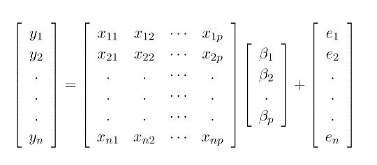
Consider the 'fixed effects' models that we have studied so far.

 are unknown, fixed effects parameters that we want to
estimate (e.g. trt1, trt2,...,trtp) and
the e1, e2,..., en are unknown, independent
and identically distributed normal (Gaussian) random variables with a mean
of Zero and a variance se2. So:
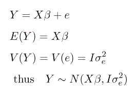
For a mixed model, we can seperate the 'fixed effects' into X and the 'random effects' into Z, thus:
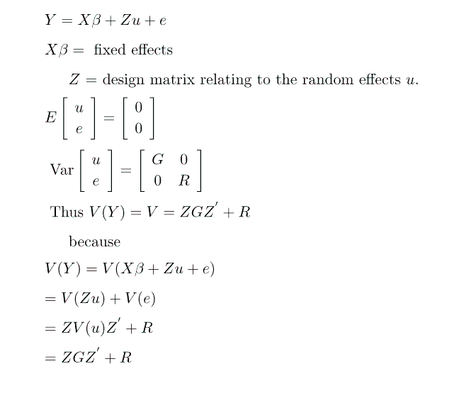
We want to estimate the parameters  , but we must
also estimate G and R . If we assume that u and e
are normally distributed we can use restricted maximum likelihood
(REML) methods to maximize the log likelihood.

To maximize this objective function we use the mixed model equations
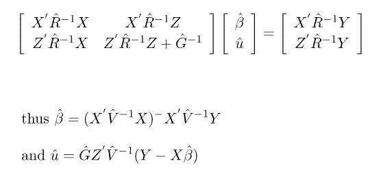
In terms of modelling the variance-covariance structure it is a good idea to have some ideas about the form of the relationships; this can be from a theoretical basis and/or by plotting the data.
The Mark 1 ocular estimation device is still unparalleled as an analytical tool!
Consider a relatively simple situation; we have 2 diets and we feed these diets to 10 sows, 5 on each diet, during their gestation and lactation. We weigh the piglets at weaning. The object of the study is to test which diet is best; best in the sense of giving us heaviest piglets at weaning.
Sows are nested within diet, since each sow is on only 1 diet. The statistical model is therefore:
where µ = effect of the mean
di = effect of the ith diet, i = 1,2
sowij = effect of the jth sow on the ith diet
pigletijk = effect of the kth piglet from the jth sow on the ith diet
eijk = effect of the random residual error associated with the measurement on the kth piglet from the jth sow on the ith diet
Up to this point we have not specified which effects are fixed and which are random; nor have we specified any covariance structure amongst random effects. We will suppose that the sows used are a representative, random sample of sows from the population of all sows. We want our sows to be a random representative sample so that our results (comparing diets) will be applicable to all sows (for other producers and sows). If our sows were not random then the results would be applicable to these sows only; not terribly useful! So we will specify the statistical distribution for sows, piglets and the residual.
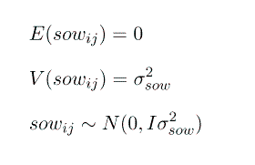
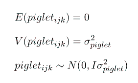
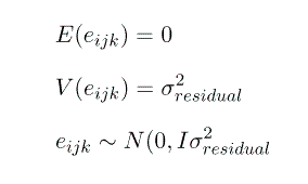
However, unfortunately, with only one measurement on each piglet we cannot seperate the effect of piglet from the effect of the residual error and we must combine them into 1 random effect. So we will redefine our random effect, e, to be
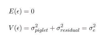
Thus in matrix notation we have
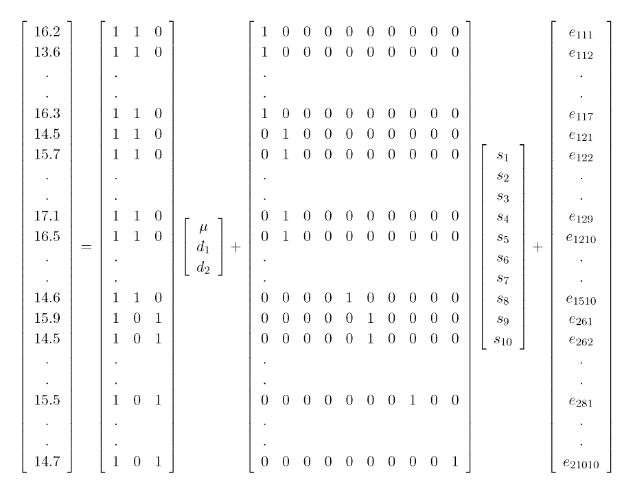
where Y = dependendent variable; piglet weaning weight (Nx1)
X = design matrix associated with the fixed effects, µ, and diets ( d1 and d2 ) (Nx3)
b = vector of unknown fixed effects parameters (µ , d1, d2 ) to be estimated (3x1)
Z = design matrix associated with the random effects of sows, sow1, sow2, ..., sow10 (Nx10)
u = vector of unknown sow effects. Note that the elements of u are not parameters (in contrast to the case for fixed effects), rather they are realisations of random variables sampled from a sow population with a distribution

e = vector of random residuals, like the elements of u they are not parameters, but rather they too are realisations of random variables, sampled from a population with a distribution

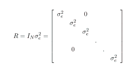
Note that this formulation gives us G = I s2sow and R = I s2e.
Observations (weaning weight)
| Diet 1 | Sow 1 | 16.2 | 13.6 | 11.1 | 15.9 | 16.6 | 14.5 | 16.3 | |||
| Sow 2 | 14.5 | 15.7 | 16.2 | 17.2 | 15.3 | 15.1 | 16.4 | 16.6 | 17.1 | 16.5 | |
| Sow 3 | 17.1 | 17.2 | 16.2 | 19.1 | 17.6 | 19.4 | 21.6 | 18.7 | 16.2 | ||
| Sow 4 | 15.5 | 16.5 | 14.8 | 15.0 | 16.7 | 14.7 | 15.3 | 15.6 | 18.2 | ||
| Sow 5 | 17.5 | 15.2 | 15.9 | 15.9 | 15.5 | 15.0 | 15.0 | 16.1 | 16.4 | 14.6 | |
| Diet 2 | Sow 6 | 15.9 | 14.5 | 12.4 | 14.7 | 15.5 | 13.2 | 14.3 | 15.1 | 15.3 | |
| Sow 7 | 14.4 | 14.8 | 13.1 | 13.4 | 13.0 | 12.2 | 13.2 | 13.5 | 13.6 | 14.7 | |
| Sow 8 | 15.5 | 15.7 | 16.0 | 14.9 | 14.9 | 14.6 | 16.1 | 13.7 | |||
| Sow 9 | 13.9 | 13.7 | 12.1 | 13.7 | 14.0 | 15.1 | 13.7 | 15.6 | 14.4 | ||
| Sow 10 | 13.4 | 13.8 | 13.2 | 12.3 | 14.0 | 11.5 | 12.7 | 13.1 | 12.5 | 14.7 |
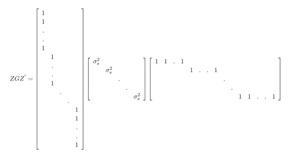
What will Y = X b+ Z u + e look like?

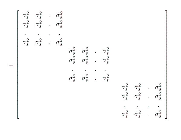
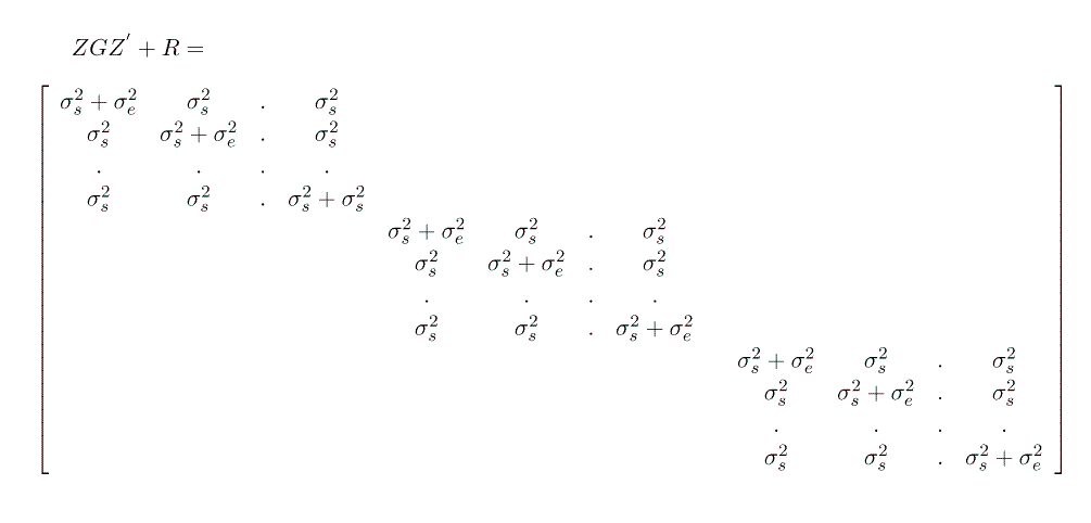
What will V(Y) look like?
data piglet;
input diet sow wwt;
cards;
1 1 16.2
1 1 13.6
1 1 11.1
1 1 15.9
1 1 16.6
1 1 14.5
1 1 16.3
1 2 14.5
1 2 15.7
1 2 16.2
1 2 17.2
1 2 15.3
1 2 15.1
1 2 16.4
1 2 16.6
1 2 17.1
1 2 16.5
1 3 17.1
1 3 17.2
1 3 16.2
1 3 19.1
1 3 17.6
1 3 19.4
1 3 21.6
1 3 18.7
1 3 16.2
1 4 15.5
1 4 16.5
1 4 14.8
1 4 15.0
1 4 16.7
1 4 14.7
1 4 15.3
1 4 15.6
1 4 18.2
1 5 17.5
1 5 15.2
1 5 15.9
1 5 15.9
1 5 15.5
1 5 15.0
1 5 15.0
1 5 16.1
1 5 16.4
1 5 14.6
2 6 15.9
2 6 14.5
2 6 12.4
2 6 14.7
2 6 15.5
2 6 13.2
2 6 14.3
2 6 15.1
2 6 15.3
2 7 14.4
2 7 14.8
2 7 13.1
2 7 13.4
2 7 13.0
2 7 12.2
2 7 13.2
2 7 13.5
2 7 13.6
2 7 14.7
2 8 15.5
2 8 15.7
2 8 16.0
2 8 14.9
2 8 14.9
2 8 14.6
2 8 16.1
2 8 13.7
2 9 13.9
2 9 13.7
2 9 12.1
2 9 13.7
2 9 14.0
2 9 15.1
2 9 13.7
2 9 15.6
2 9 14.4
2 10 13.4
2 10 13.8
2 10 13.2
2 10 12.3
2 10 14.0
2 10 11.5
2 10 12.7
2 10 13.1
2 10 12.5
2 10 14.7
;

proc mixed data=piglet;
class diet sow;
model wwt = diet/s;
random sow(diet);
estimate 'Diet 1' intercept 1 diet 1 0;
estimate 'Diet 2' intercept 1 diet 0 1;
estimate 'D1 - D2' diet 1 -1;
run;
quit;
The SAS System
                              The MIXED Procedure

                            Class Level Information

                      Class     Levels  Values
                      DIET           2  1 2
                      SOW           10  1 2 3 4 5 6 7 8 9 10
                      REML Estimation Iteration History

              Iteration  Evaluations     Objective    Criterion
                      0            1  159.7096
                      1            2  138.2057      0.00000005
                      2            1  138.2043      0.00000003
                      3            1  138.2043      0.00000000

                         Convergence criteria met.
                   Covariance Parameter Estimates (REML)

                   Cov Parm       Estimate
                   SOW(DIET)  0.8833     s2sow
                   Residual      1.3400
Model Fitting Information for WWT
                 Description                      Value
              Observations                        91.0000
              Res Log Likelihood                -150.888
              Akaike's Information Criterion    -152.888
              Schwarz's Bayesian Criterion      -155.376
              -2 Res Log Likelihood              301.7754
Solution for Fixed Effects
   Effect     Estimate     Std Error  DF  t      Pr > |t|
   INTERCEPT  14.08220470  0.45382186 8   31.03  0.0001
   DIET 1     2.04401332   0.64250396 8    3.18  0.0130
   DIET 2     0.00000000    .         .     .     .
Tests of Fixed Effects
    Source     NDF   DDF    Type III F    Pr > F


    DIET        1     8     10.12         0.0130
ESTIMATE Statement Results
Parameter Estimate Std Error DF t Pr > |t|
 Diet 1    16.12621803  0.45481540   8   35.46   0.0001
 Diet 2    14.08220470  0.45382186   8   31.03   0.0001
 D1 - D2    2.04401332  0.64250396   8    3.18   0.0130
Implicit in our model description is the understanding that, conditional upon the dam, all the piglets in a litter are independent of oneanother:
We can test whether a variance component contributes significantly to the model and hence whether it should be retained.
Formally, the model we have fitted has the random parameters s2sow and s2e . If we consider this the ``Full Model'' then the log likelihood LnLF has parameters b, s2sow, s2e . If we drop the parameter s2sow (equivalent to setting s2sow = 0) then we have a ``Reduced Model'' and the log likelihood LnLR has parameters b, s2e . Thus the reduced model is a subset of the full model. From Maximum Likelihood theory it can be shown that -2 the difference in the log likelihoods has a c2 distribution with expectation equal to the number of degrees of freedom associated with the difference in the number of estimable parameters in the two models (the Full and Reduced).
Therefore, if we fit a model without sow we will have 1 less parameter ( s2sow ). The difference in the log likelihoods can therefore be used to test whether the sow variance has a statistically significant effect and hence should be retained in the model.
If we fit this reduced model we find:
proc mixed data=piglet;
class diet sow;
model wwt = diet/s;
estimate 'Diet 1' intercept 1 diet 1 0;
estimate 'Diet 2' intercept 1 diet 0 1;
estimate 'D1 - D2' diet 1 -1;
run;
quit;
The SAS System
                              The MIXED Procedure

                            Class Level Information

                      Class     Levels  Values
                      DIET      2  1 2
                      SOW       10     1 2 3 4 5 6 7 8 9 10
Covariance Parameter Estimates (REML)
                  Cov Parm          Estimate
                  Residual            2.03134973    s2e
Model Fitting Information for WWT
                  Description                     Value
                Observations                      91.0000
                Res Log Likelihood              -161.640
                Akaike's Information Criterion  -162.640
                Schwarz's Bayesian Criterion    -163.885
                -2 Res Log Likelihood            323.2807
Solution for Fixed Effects
    Effect       Estimate     Std Error    DF   t     Pr > |t|
   INTERCEPT   14.03478261    0.21014228   89  66.79  0.0001
   DIET 1       2.12743961    0.29883253   89   7.12  0.0001
   DIET 2       0.00000000     .            .    .     .
                 Tests of Fixed Effects

       Source     NDF  DDF   Type III F    Pr > F
DIET 1 89 50.68 0.0001
                ESTIMATE Statement Results

    Parameter     Estimate    Std Error    DF   t      Pr > |t|
  Diet 1       16.16222222   0.21246436    89   76.07   0.0001
  Diet 2       14.03478261   0.21014228    89   66.79   0.0001
  D1 - D2       2.12743961   0.29883253    89    7.12   0.0001
| -2 LnLR | 323.2807 |
| -2 LnLF | 301.7754 |
| Difference | 21.5053 |
This is for 1 d.f. Suppose we have decided that we will use a 95% probability level so that we are running the risk of a Type I error 5% of the time. The critical tabulated value for c21 d.f.,5% is 3.841. Since the difference (21.5053) surpasses this we can conclude that the effect of sow (the sow variance) is statistically signficant, i.e. that s2sow > 0 and that we should retain s2sow as a parameter in the model.
We have looked at the above example as measurements on the piglets where we account for the sow variance. However, we can also (and equivalently) look at the measurements as repeated measurements on the sows. If we consider that we have repeated measurements with a compound symmetry structure (the correlation between any pair of records is the same) then we get:
proc mixed data=piglet;
class diet sow;
model wwt = diet/s;
repeated /type=cs sub=sow(diet) r rcorr;
estimate 'Diet 1' intercept 1 diet 1 0;
estimate 'Diet 2' intercept 1 diet 0 1;
estimate 'D1 - D2' diet 1 -1;
run;
quit;
This will give us exactly the same results as for the random model, the two are equivalent.
We will suppose that we have test-day production records on a number of dairy cows, all kept in the same herd, of various parities. We record the stage of lactation (Days-In-Milk) when each test is made and we record various production parameters (milk, fat and protein yields, fat % and protein %, Somatic Cell Count, Total Enery , Protein and Dry Matter consumption as well as Basal Enery, Protein and DM intake, and Milk Value and Feed Costs). We could use a simple random effects model, of each cow, supposing that all test-day records of a cow are equally correlated. Cows are from various parities, so cow is nested within parity (our data are only for 1 lactation).
The following code shows the SAS statements to read in the external file with the test-day records.
data repeat1;
infile '\repeated\tdrecs.dat' lrecl=180;
input  cow 7-12  parity 55-56  iage 57-60  idim 61-64 milk 65-70
 fat 71-76 protein;
 dim = idim;
run;
proc mixed data=tday;
class parity cow idim;
model milk = parity/s;
random cow(parity);
run;
quit;
According to our knowledge of dairy cattle this is probably a somewhat simplistic model since we might reasonably suppose that test-day records are not all equally correlated. The further apart test-day records are, the less correlated they are likely to be. However, it will serve as a base against which to compare models and build up more complex formulations.
We could use a simple compound symmetry repeated measures model, which will be exactly the same as the random effects model we have examined, as discussed in the sow/piglet model.
proc mixed data=tday;
class parity cow idim;
model milk = parity/s;
repeated idim/type=cs sub=cow(parity) r rcorr;
run;
quit;
In the repeated statement we specify idim because this indicates the days-in-milk; cows are not all milked on the same days in milk and not all cows have exactly the same number of tests. The subject specifies that the compound symmetry structure applies to submatrices corresponding to each SUBject. The SUBject designation comes from the historical development of repeated measurements in human psychology where individuals are often refered to as subjects.
This model is not any better than the random model; it is just a re-formulation as a repeated measures model.
If we want to fit a model with the desired property that observations closer together are more highly correlated and observations further apart are less correlated then an autoregressive covariance structure may be appropriate, AR(1). This expresses the covariance between observations as s2 rw , where w is the number of time intervals between the observations. This assumes that the time intervals are equal and the same for all individuals (SUBjects); for example that measurements were made at 1, 2, 3, 4, 5, 6 hours, etc.
proc mixed data=tday;
class parity cow idim;
model milk = parity/s;
repeated idim/type=ar(1) sub=cow(parity) r rcorr;
run;
quit;
In many biological experiments the time intervals may not be equal, in which case an AR(1) model may well not be appropriate.
As noted above, it is often sensible to consider some sort of time-series covariance structure, such that the correlations of the repeated measurements are assumed to be smaller for observations that are further apart, in a spatial or temporal sense. This is where spatial structures enter and is the basis of spatial and temporal statistics; common in geology and related sciences. Their development has been for spatial separation; however, we can view unequally spaced time data as a spatial process in one dimension (that of time). In SAS the SP(POW) structure for unequally spaced data provides a direct generalisation of the AR(1) structure for equally spaced data. SP(POW) models the covariance between two measurements and times T1 and T2 as
proc mixed data=tday;
class parity cow idim;
model milk = parity/s;
repeated idim/type=sp(pow)(dim) sub=cow(parity) r rcorr;
run;
quit;
We can build up and compare the various models, in terms of the variance-covariance structure, since the fixed effects component is the same in each case.
| -2 LnLR | |
| s2e | 695.4845 |
| s2cow + s2e (random) | 692.5492 |
| compound symmetry | 692.5492 |
| AR(1) | 695.4845 |
| Spatial Power | 605.7209 |
A brief note is added here to indicate that another possibility may be to use 'Random Regressions' models. Such models are outside of the scope of this course, but are discussed in the SAS System for Mixed Models book, and in a genetic context are addressed in the book by Mrode (Linear models for the prediction of animal breeding values, 2nd Edition) and in various scientific papers by authors such as Karin Meyer (Australia) and Larry Schaeffer (Guelph).