Another possibility is what is commonly called a Randomised Complete Block (RCB) design.

Suppose that we had 4 varieties of maize that we wish to compare. We decide to carry out this test at 12 random locations ('blocks') throughout the St-Lawrence valley; so that the results will be considered as being applicable to the maize-growing region of the St-Lawrence. At each location we have a field and we allocate 4 plots; each variety of maize is grown in a seperate plot, randomly assigned at each location.

This would be a RCB, at each block/location we assign each variety of maize to a plot at random; hence the name Randomised Complete Block.

Another example looking at animals might be to compare the effects of 4 diets for growing pigs. We are going to be making detailed feed consumption/digestion studies and the animals will be kept in the Macdonald Animal Facilities, which have a fairly stable environment throughout the year. Unfortunately we only have 4 pens and this is all that we are able to manage at once; in terms of feeding, sampling, lab analyses, etc. Even graduate students have to sleep and study other things; like statistics courses! The growing pigs will be kept for approximately 1 month in the pens. So what we decide to do is, each month we will put 4 pigs in the individual pens and randomly assign them 1 to each of the 4 diets. The following month another 4 pigs will be used. Thus over the course of a year (12 months) we will have 12 'blocks' and 48 pigs, 12 on each diet, 4 pigs in each 'block'/month, 1 per diet. We will consider the 'blocks' as random, since we are not interested in the specific month effects and since the Animal Facilities are kept at a uniform environment then any small variations from month to month are random.

For either of these two scenarios we obtain the following data :

Weight gain in pigs/Maize Yield

Variety	Location	Maize Yield
Diet	Month	Piglet Wt Gain
1	1	51.9
2	1	53.7
3	1	54.9
4	1	55.6
1	2	51.6
2	2	50.9
3	2	52.2
4	2	53.8
1	3	44.0
2	3	46.0
3	3	47.3
4	3	48.4
1	4	52.6
2	4	52.8
3	4	54.0
4	4	56.3
1	5	56.5
2	5	57.5
3	5	58.2
4	5	61.7
1	6	48.5
2	6	50.8
3	6	51.6
4	6	52.0
1	7	52.1
2	7	53.4
3	7	55.5
4	7	56.1
1	8	52.6
2	8	52.4
3	8	53.6
4	8	55.8
1	9	49.3
2	9	49.4
3	9	52.1
4	9	51.6
1	10	51.1
2	10	52.5
3	10	52.9
4	10	57.1
1	11	58.6
2	11	57.6
3	11	58.9
4	11	61.0
1	12	45.1
2	12	46.7
3	12	47.9
4	12	48.0

A suitable model would be

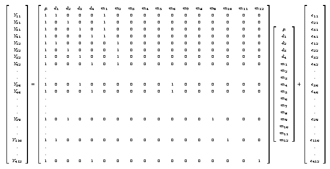
Y_ij = µ + diet_i + month_j + pen_ij + animal_ij + e_ij

As before, we have only 1 observation for each animal and hence pen_ij, animal_ij and residual_ij are confounded and cannot be seperated; so that

e_ij = pen_ij + animal_ij + residual_ij

So our model becomes

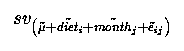
Y_ij = µ + diet_i + month_j + e_ij

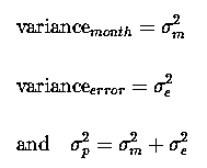
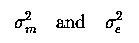
But what are the parameters of our model? µ and diet are fixed effects. Both month and e are random effects, with variances :

We can set up our equations in a similar manner as before, Y = Xb + e.

However, what we have is what is called a 'mixed' model. We have a 'fixed' effect (diet) and a 'random' effect (month).

We will analyse this using SAS PROC MIXED, whereby we can specify which effects are fixed and which are random.

data rcb2;
input diet month gain;
cards;
...
...
;

proc mixed;
classes diet month;
model gain = diet;
random month;
lsmeans diet;
estimate 'mean + diet 1' intercept 1 diet 1 0 0 0;
estimate 'mean + diet 2' intercept 1 diet 0 1 0 0;
estimate 'mean + diet 3' intercept 1 diet 0 0 1 0;
estimate 'diet 1 - 2'  diet 1 -1 0 0;
estimate 'diet 1 - 3'  diet 1 0 -1 0;
run;

Note that we specified that diet and month are classes (qualitative levels and not quantitative values).

In the model statement we have gain, our dependent variable = diet (our fixed effect). We do NOT specify the random effect(s), only the fixed effect(s) in the model statement.

With the random statement we define that month is to be included and considered as a random effect.

Unlike PROC GLM, for fixed effects models, PROC MIXED is an iterative method and uses Restricted Maximum Likelihood (REML) for estimating the fixed effects and the random variance components .

See 'SAS System for Mixed Models' for a VERY good introduction to Mixed Models.

For our estimate of µ + diet 1 we obtain 51.1583 ± 1.1236.

How did this arise?

We know that a fitted value corresponding to an observation is estimable.

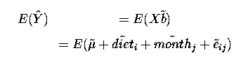
But month and e are both random effects and hence have an expectation of Zero. Hence we have an estimate of .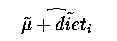

What is the sampling variance to our estimate?

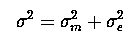
When we had only a fixed effects model, be it regression or classification we said that the real, fixed effects had no error and that the only variance came from the random effect(s), the error (residual).

Now we have that both month and e are random; hence i.e. 14.544886 + 0.6041477 = 15.149033.

We have 12 observations for diet 1, so the sampling variance is , 15.149033/12 = 1.2624

Then as always, our standard error is simply the square root of the sampling variance, which gives us 51.1583 ± 1.1236.

If we look at differences between diets we have a slightly different view. The difference between fitted values is estimable; so let us estimate the difference between diet 1 and diet 2;

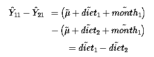
Thus the difference between diets does not involve the month effects and we find that the sampling variance for diet differences involves only the residual variance.

PROC MIXED handles all of these transparently. It uses the correct, appropriate variances as needed; we might say that it does all this 'automagically'!

To see whether the effect of Month is statistically significant we can re-run our model but dropping out the random effect of Month and then examine the difference in the -2 Log Likelihood. See the link at the bottom of this page for the Results/Output/Interpretation.

To illustrate the importance of treating the random effects properly let us consider what would be the result if we had simply used the traditional fixed effects type ANOVA/Least Squares approach as exemplified by using PROC GLM.

We would have :

proc glm;
classes diet month;
model gain = diet month;
random month;
lsmeans diet/stderr;
estimate 'mean diet 1' intercept 12 diet 12 0 0 0
  month 1 1 1 1 1 1 1 1 1 1 1 1/divisor=12;
estimate 'mean diet 2' intercept 12 diet 0 12 0 0
  month 1 1 1 1 1 1 1 1 1 1 1 1/divisor=12;
estimate 'd1 - d2' diet 1 -1 0 0;
estimate 'd1 - d3' diet 1 0 -1 0;
run;
quit;

What we find is that PROC GLM ignores the variance due to month when calculating the sampling variances (and standard errors) to our Least Squares means and estimates.

This is because PROC GLM is a fixed effects model, notwithstanding that we claimed that month was a random effect. GLM is in fact schizophrenic in this regard; it fits everything as a fixed effects model and then when we say that month is a random effect it goes and computes the expectations of the mean squares with month as random!

This illustrates the danger of miss-using a statistical package. Many, many data from RCB's have been analysed using SAS PROC GLM, and most other statistical programs : inappropriately. A common theme was that until recently computers were not powerful enough to handle mixed models adequately. This limitation is largely obviated now.

If you have a mixed model design then you should analyse it as a proper mixed model! Anything other than a mixed model will likely mean that the sampling variance (of you) is seriously underestimated (referees will reject the papers you submit for publication!).

Output, results and explanations of the above SAS analyses

Suppose we are carrying out an experiment to compare 2 diets being fed to young piglets (immediately post-weaning). In order to minimize the residual variance, and since we know that there are likely to be effects of the sow(s) (the dams of the young piglets), we decide to use pairs of piglets from several sows, and to randomly assign the pairs of pigs one to each diet.

Such data are often analysed using a paired t-test, the idea being that the differences between the sows do not affect the differences between the piglets due to the diets.

Consider the following data from pairs of piglets from 16 sows.

Weight gain in piglets

	Weight	Gain
Sow	Diet A	Diet B
1	37.02	47.94
2	40.13	50.24
3	34.12	.
4	36.02	50.26
5	42.03	53.81
6	41.92	53.86
7	36.57	.
8	39.53	51.71
9	38.53	52.68
10	36.02	43.58
11	37.54	39.03
12	.	51.87
13	40.77	48.63
14	41.66	55.91
15	45.20	57.38
16	37.88	46.37

We note that 3 piglets were lost, 2 from Diet B and one from Diet A.

Below we see various analyses: a paired t-test (which I abhor) as well as analyses using proc mixed.

data paired1;
input sow DietA DietB;
diff = DietA - DietB;
cards;
   1     37.02    47.94
   2     40.13    50.24
   3     34.52     .
   4     36.02    50.26
   5     42.03    53.81
   6     41.92    53.86
   7     36.57     .
   8     39.43    51.71
   9     38.53    52.68
  10     36.02    43.58
  11     37.54    39.03
  12      .       51.87
  13     40.77    48.63
  14     41.66    55.91
  15     45.20    57.38
  16     37.88    46.37
;

proc ttest data=paired1; <- bad
 paired DietA*DietB;
run;

proc glm data=paired1;
model diff =;
run;
quit;


data paired2;
input sow Diet $ WtGain;
cards;
   1 A    37.02
   1 B    47.94
   2 A    40.13
   2 B    50.24
   3 A    34.52
   3 B     .
   4 A    36.02
   4 B    50.26
   5 A    42.03
   5 B    53.81
   6 A    41.92
   6 B    53.86
   7 A    36.57
   7 B     .
   8 A    39.43
   8 B    51.71
   9 A    38.53
   9 B    52.68
  10 A    36.02
  10 B    43.58
  11 A    37.54
  11 B    39.03
  12 A     .
  12 B    51.87
  13 A    40.77
  13 B    48.63
  14 A    41.66
  14 B    55.91
  15 A    45.20
  15 B    57.38
  16 A    37.88
  16 B    46.37
;

proc mixed data=paired2;  <- good
class sow Diet;
model WtGain = Diet/ddfm=kr;
random sow;
lsmeans Diet/pdiff adjust=bon;
estimate 'Diet A-B' Diet 1 -1;
run;

proc mixed data=paired2;
class sow Diet;
model WtGain = Diet/ddfm=kr;
run;

In a paired t-test, we must have the observations on both pairs, consequently the observations from the piglets from sows 3, 7 and 12 must be discarded. Thus a paired t-test is not able to make use of any information from these unpaired observations. In addition, the reason we decided to use a paired t-test is because we think/know/suspect that there may be differences amongst the 'blocking' factors, i.e. the sows in this case. BUT, our analysis is not able to give us any information about this aspect.

Our paired t-test estimates the difference (A-B) as -10.5577 +/- 0.9877; which difference is highly statistically significant.

A better method of analysis is the analysis using proc mixed; we make use of ALL the observations, including the unpaired observations. This means we actually end up with more information to estimate the difference A-B. In addition we also obtain an estimate of the between-block variance, i.e. the variation amongst sows. This was the reason for the blocking (pairs of piglets from sows), and provides statistical evidence as to whether this was a sensible strategy, as well as being biologically interesting in its own right. So, even though the primary objective of our study may be to look at the difference between treatment A and treatment B, we also have some other interesting and useful results; the biological variability amongst sows. This will be useful to other, future researchers to allow and help them in designing their experiments and in knowing whether there are likely to be substantive differences amongst sows.

So; what do we get with our analysis using proc mixed? We fidn that the residual variance is 6.2733, and the variance amongst sows is 9.5491; i.e. there do seem to be important differences amongst sows. The estimate of the difference (A-B) is -10.8334 +/- 0.9689. The estimates from the paired t-test and proc mixed are not hugely different; however, the analysis from proc mixed is the better analysis (and has a slightly smaller standard error) as well as providing an estimate of the between-sow variance, which the paired t-test does not do.

Moral of this? Do not use a paired t-test, there are better analyses, and I shall castigate you if you use a paired t-test. The only reason for a paired t-test is that it is easy to calculate by hand. Hence before computers and statistical software (such as SAS and R) were ubiquitous it was an acceptable method; we HAVE progressed in the past 40 years!