This is a first attempt at an R version of the SAS two-way, fixed effects model.
Data file with recorded observations
R code to read in the data and carry out the Two-Way Fixed effects analysis
Mocel 1, fitting Diet+Parity, we use the following code,and get the below results.
> lm1 <-lm(y~Diet+Parity,data=ds)
> lm1

Call:
lm(formula = y ~ Diet + Parity, data = ds)

Coefficients:
(Intercept)        Diet2        Diet3        Diet4        Diet5
     3.4320      -0.3286      -0.6096       2.0904       1.4404
      Diet6      Parity2      Parity3      Parity4
     2.4154       0.5064       2.7207       1.4833

> anova(lm1)
Analysis of Variance Table

Response: y
          Df Sum Sq Mean Sq F value   Pr(>F)
Diet       5 35.619  7.1237  5.3546 0.006864 **
Parity     3 22.096  7.3652  5.5360 0.011347 *
Residuals 13 17.295  1.3304
---
Signif. codes:  0 ‘***’ 0.001 ‘**’ 0.01 ‘*’ 0.05 ‘.’ 0.1 ‘ ’ 1
>
From this we can see that the degrees of freedom, Marginal (Type III) Sums of Squares, Mean Squares, F value and Prob for the effect of Parity are :
          Df Sum Sq Mean Sq F value   Pr(>F)
Parity     3 22.096  7.3652  5.5360 0.011347 *
Similarly, re-fitting the model, but with the order reversed will give us the Marginal effects of Diet (i.e. over and above te effects of Parity):
> # fitting Parity+Diet, to get R(D|mu,P)
> lm2 <-lm(y~Parity+Diet,data=ds)
> lm2

Call:
lm(formula = y ~ Parity + Diet, data = ds)

Coefficients:
(Intercept)      Parity2      Parity3      Parity4        Diet2
     3.4320       0.5064       2.7207       1.4833      -0.3286
      Diet3        Diet4        Diet5        Diet6
    -0.6096       2.0904       1.4404       2.4154

> anova(lm2)
Analysis of Variance Table

Response: y
          Df Sum Sq Mean Sq F value   Pr(>F)
Parity     3 25.861  8.6204  6.4795 0.006435 **
Diet       5 31.853  6.3706  4.7885 0.010593 *
Residuals 13 17.295  1.3304
---
Signif. codes:  0 ‘***’ 0.001 ‘**’ 0.01 ‘*’ 0.05 ‘.’ 0.1 ‘ ’ 1
>
From this we can see that the degrees of freedom, Marginal (Type III) Sums of Squares, Mean Squares, F value and Prob for the effect of Diet are :
          Df Sum Sq Mean Sq F value   Pr(>F)
Diet       5 31.853  6.3706  4.7885 0.010593 *
Our final model (lm3) will allow us to compute the effect of the Model over and above the Mean:
> # fitting mu, to get R(|mu), and hence R(D,P|mu)
> lm3 <-lm(y~1,data=ds)
> lm3

Call:
lm(formula = y ~ 1, data = ds)

Coefficients:
(Intercept)
      5.495

> anova(lm3)
Analysis of Variance Table

Response: y
          Df Sum Sq Mean Sq F value Pr(>F)
Residuals 21  75.01  3.5719
>
Thus we can compute the effect of the Model over and above the mean, R(D,P| µ) as:
SS (D,P| µ) = 75.01 - 17.295 = 57.715
df (D,P| µ) = 21 - 13 = 8
This therefore gives us our usual Analysis of Variance
| Source of variation | d.f. | Sums of Squares | Mean Squares | F-ratio | Prob. |
|---|---|---|---|---|---|
| Total | N = 22 | 739.3 | |||
| Model | r(X) = 9 | 722.0055 | 8.0 | 6.014 | |
| C.F. mean | 1 | 664.29055 | 664.29055 | 487.1 | |
| Model after µ, R(Diet, Parity|µ ) | r(X)-1 = 8 | 57.715 | 7.214 | 5.422 | |
| Parity, R(Parity|µ, Diet ) | 3 | 22.096 | 7.3652 | 5.5360 | .01135 |
| Diet, R(Diet|µ, Parity ) | 5 | 31.853 | 6.3706 | 4.7885 | .01059 |
| Residual | N-r(X) = 13 | 17.295 | 1.3304 |
We are using a 5% probability level as our criteria for accepting/rejecting our Null Hypotheses. Consequently we shall conclude that there are statistically significant effects of both Parity and Diet.
In the above models we ask to output the lm object; one of the terms of the lm object is the solution vector. Consider the object lm1: we have
lm(formula = y ~ Diet + Parity, data = ds)

Coefficients:
(Intercept)        Diet2        Diet3        Diet4        Diet5
     3.4320      -0.3286      -0.6096       2.0904       1.4404
      Diet6      Parity2      Parity3      Parity4
     2.4154       0.5064       2.7207       1.4833
We see that there is nothing for Diet 1, nor for Parity 1. How come? Well, If we had included Diet 1 then we would have not had a full-rank subset matrix. Likewise, if we include the effect of Parity 1 then the design matrix would not be of full rank. So, R sets the values of the first level of each fixed effect to Zero, and then omits them from the model (and solution vector). This is in contrast to SAS (proc glm et al) where the last level of each fixed effect is set to Zero, but not omitted from the model. Both approaches are statistically equivalent, and as long as we are careful to keep track of what is what then we shall obtain exactly the same answer for the same question. One drawback with R, is that the terms in the solution vector are all estimates, but maybe not always quite what you might simply think by just looking at the names of the terms of the solution vector, particularly if there are nested terms in a model or if there are interactions. A consequence of this is that it is easy to estimate something which may not be quite what you actually want or meant; caveat emptor!
Fitted values are always estimable. Fitted values are the estimated values corresponding to the actual observations we have. So, here, in this analysis we have 22 observations (2 of the original observations are missing, for reasons which are completely unrelated to the experiment, and hence are MAR [missing at random]). We can set up a coefficient matrix and use the ESTICON function from the doBy package to estimate the 22 fitted values, and also other functions of these fitted values. NOTE; I have specified (below) the coefficient matrices (w1) with extra spaces between the different 'parts' of the solution vector, to make it easier (for me, and hopefully for you too) to see which coefficents refer to which terms of the solution vector.
> # explicitly estimate fitted values
> # pay attention to the (full-rank) solution vector
> #
> # mu + diet_1 + parity_1
> w1<-c(1, 0,0,0,0,0, 0,0,0)
> esticon(lm1,w1)
  beta0 Estimate Std.Error t.value DF  Pr(>|t|)    Lower    Upper
1     0 3.431994 0.7732346 4.43849 13 0.0006686 1.761522 5.102466
>
> # NOTE diet_1 parity_2 is missing
>
> # mu + diet_1 + parity_3
> w1<-c(1, 0,0,0,0,0, 0,1,0)
> esticon(lm1,w1)
  beta0 Estimate Std.Error t.value DF Pr(>|t|)    Lower    Upper
1     0 6.152679 0.7859322 7.82851 13  2.8e-06 4.454775 7.850582
>
> # mu + diet_1 + parity_4
> w1<-c(1, 0,0,0,0,0, 0,0,1)
> esticon(lm1,w1)
  beta0 Estimate Std.Error  t.value DF Pr(>|t|)    Lower    Upper
1     0 4.915327 0.7732346 6.356838 13 2.51e-05 3.244856 6.585799
>
> # mu + diet_2 + parity_1
> w1<-c(1, 1,0,0,0,0, 0,0,0)
> esticon(lm1,w1)
  beta0 Estimate Std.Error  t.value DF Pr(>|t|)    Lower    Upper
1     0 3.103423 0.7732346 4.013559 13 0.001474 1.432951 4.773894
>
> # mu + diet_2 + parity_2
> w1<-c(1, 1,0,0,0,0, 1,0,0)
> esticon(lm1,w1)
  beta0 Estimate Std.Error  t.value DF Pr(>|t|)    Lower    Upper
1     0 3.609821 0.7859322 4.593044 13 0.000504 1.911918 5.307725
>
> # NOTE diet_2 parity_3 is missing
>
> # mu + diet_2 + parity_4
> w1<-c(1, 1,0,0,0,0, 0,0,1)
> esticon(lm1,w1)
  beta0 Estimate Std.Error  t.value DF Pr(>|t|)    Lower    Upper
1     0 4.586756 0.7732346 5.931907 13 4.97e-05 2.916284 6.257228
>
> # mu + diet_3 + parity_1
> w1<-c(1, 0,1,0,0,0, 0,0,0)
> esticon(lm1,w1)
  beta0 Estimate Std.Error  t.value DF  Pr(>|t|)    Lower    Upper
1     0 2.822396 0.7112188 3.968393 13 0.0016049 1.285901 4.358891
>
> # mu + diet_3 + parity_2
> w1<-c(1, 0,1,0,0,0, 1,0,0)
> esticon(lm1,w1)
  beta0 Estimate Std.Error  t.value DF  Pr(>|t|)    Lower    Upper
1     0 3.328795 0.7331498 4.540402 13 0.0005548 1.744921 4.912668
>
> # mu + diet_3 + parity_3
> w1<-c(1, 0,1,0,0,0, 0,1,0)
> esticon(lm1,w1)
  beta0 Estimate Std.Error  t.value DF Pr(>|t|)    Lower    Upper
1     0  5.54308 0.7331498 7.560638 13  4.1e-06 3.959207 7.126954
>
> # mu + diet_3 + parity_4
> w1<-c(1, 0,1,0,0,0, 0,0,1)
> esticon(lm1,w1)
  beta0 Estimate Std.Error  t.value DF Pr(>|t|)    Lower    Upper
1     0 4.305729 0.7112188 6.054014 13 4.07e-05 2.769234 5.842224
>
> # mu + diet_4 + parity_1
> w1<-c(1, 0,0,1,0,0, 0,0,0)
> esticon(lm1,w1)
  beta0 Estimate Std.Error  t.value DF Pr(>|t|)    Lower    Upper
1     0 5.522396 0.7112188 7.764693 13  3.1e-06 3.985901 7.058891
>
> # mu + diet_4 + parity_2
> w1<-c(1, 0,0,1,0,0, 1,0,0)
> esticon(lm1,w1)
  beta0 Estimate Std.Error  t.value DF Pr(>|t|)    Lower    Upper
1     0 6.028795 0.7331498 8.223142 13  1.7e-06 4.444921 7.612668
>
> # mu + diet_4 + parity_3
> w1<-c(1, 0,0,1,0,0, 0,1,0)
> esticon(lm1,w1)
  beta0 Estimate Std.Error  t.value DF Pr(>|t|)    Lower    Upper
1     0  8.24308 0.7331498 11.24338 13        0 6.659207 9.826954
>
> # mu + diet_4 + parity_4
> w1<-c(1, 0,0,1,0,0, 0,0,1)
> esticon(lm1,w1)
  beta0 Estimate Std.Error  t.value DF Pr(>|t|)    Lower    Upper
1     0 7.005729 0.7112188 9.850314 13    2e-07 5.469234 8.542224
>
> # mu + diet_5 + parity_1
> w1<-c(1, 0,0,0,1,0, 0,0,0)
> esticon(lm1,w1)
  beta0 Estimate Std.Error  t.value DF Pr(>|t|)    Lower    Upper
1     0 4.872396 0.7112188 6.850769 13 1.17e-05 3.335901 6.408891
>
> # mu + diet_5 + parity_2
> w1<-c(1, 0,0,0,1,0, 1,0,0)
> esticon(lm1,w1)
  beta0 Estimate Std.Error  t.value DF Pr(>|t|)    Lower    Upper
1     0 5.378795 0.7331498 7.336556 13  5.7e-06 3.794921 6.962668
>
> # mu + diet_5 + parity_3
> w1<-c(1, 0,0,0,1,0, 0,1,0)
> esticon(lm1,w1)
  beta0 Estimate Std.Error  t.value DF Pr(>|t|)    Lower    Upper
1     0  7.59308 0.7331498 10.35679 13    1e-07 6.009207 9.176954
>
> # mu + diet_5 + parity_4
> w1<-c(1, 0,0,0,1,0, 0,0,1)
> esticon(lm1,w1)
  beta0 Estimate Std.Error t.value DF Pr(>|t|)    Lower    Upper
1     0 6.355729 0.7112188 8.93639 13    7e-07 4.819234 7.892224
>
> # mu + diet_6 + parity_1
> w1<-c(1, 0,0,0,0,1, 0,0,0)
> esticon(lm1,w1)
  beta0 Estimate Std.Error  t.value DF Pr(>|t|)    Lower    Upper
1     0 5.847396 0.7112188 8.221655 13  1.7e-06 4.310901 7.383891
>
> # mu + diet_6 + parity_2
> w1<-c(1, 0,0,0,0,1, 1,0,0)
> esticon(lm1,w1)
  beta0 Estimate Std.Error  t.value DF Pr(>|t|)    Lower    Upper
1     0 6.353795 0.7331498 8.666434 13    9e-07 4.769921 7.937668
>
> # mu + diet_6 + parity_3
> w1<-c(1, 0,0,0,0,1, 0,1,0)
> esticon(lm1,w1)
  beta0 Estimate Std.Error  t.value DF Pr(>|t|)    Lower    Upper
1     0  8.56808 0.7331498 11.68667 13        0 6.984207 10.15195
>
> # mu + diet_6 + parity_4
> w1<-c(1, 0,0,0,0,1, 0,0,1)
> esticon(lm1,w1)
  beta0 Estimate Std.Error  t.value DF Pr(>|t|)    Lower    Upper
1     0 7.330729 0.7112188 10.30728 13    1e-07 5.794234 8.867224
>
Pay particular attention to the coefficient matrix and how the coefficients correspond to terms in the model. Note how the term labelled Intercept (from lm1) is in fact (µ + Diet_1 + Parity_1); it is NOT (µ).
The differences amongst the pairs of Parities are estimable, since they can be expressed as a linear function of various fitted values.
we have the fitted value for
[1] mu + diet_4 + parity_1 (1, 0,0,1,0,0, 0,0,0)
[2] mu + diet_4 + parity_2 (1, 0,0,1,0,0, 1,0,0)
thus [1]-[2] = parity_1 - parity_2 (0, 0,0,0,0,0, 1,0,0)
Code and results:
> # thus parity_1 - parity_2 (0, 0,0,0,0,0, 1,0,0)
> w1<-c(0, 0,0,0,0,0, 1,0,0)
> esticon(lm1,w1)
  beta0  Estimate Std.Error   t.value DF  Pr(>|t|)     Lower    Upper
1     0 0.5063988  0.709128 0.7141148 13 0.4877808 -1.025579 2.038377
>
We can combine this with the fitted value for (mu + Diet_1 + Parity_1) to obtain an estimate of (mu + Diet_1 + Parity_2), one of our missing values :-)
> # mu + diet_1 + parity_2
> w1<-c(1, 0,0,0,0,0, 1,0,0)
> esticon(lm1,w1)
  beta0 Estimate Std.Error  t.value DF  Pr(>|t|)    Lower   Upper
1     0 3.938393 0.8987479 4.382089 13 0.0007417 1.996766 5.88002
Another place where the esticon function is useful, is when we wish to construct a custom contrast not automatically provided by regular packages (such as lsmeans). Suppose we wish and need to compute the average of Diets 1 & 2. We can use esticon for this:
# explicitly compute our lsmean for (mu + trt 1)
w1<-c(1, 0,0,0,0,0, 1/4,1/4,1/4)
esticon(lm1,w1)

# explicitly compute our lsmean for (mu + trt 2)
w2<-c(1, 1,0,0,0,0, 1/4,1/4,1/4)
lsm2<-esticon(lm1,w2)
lsm2
Then the average of these is
# explicitly compute our lsmean for (mu + [trt 1 + trt 2]/2)
w2<-c(1, 0.5,0,0,0,0, 1/4,1/4,1/4)
lsm2<-esticon(lm1,w2)
lsm2
What will be our next steps? Well we shall want to estimate various things: least squares means and differences amongst the various effects means; .e.g. differences amongst the Diet means, or differences amongst the Parity means. There are significant Diet effects, i.e the effects of Diets are not all equal. That does not mean that all the Diets differ from one another. What are the estimates of the differences, and which ones can be considered to be statistically significant?
It is very common to report least-squares maans (also called estimated/predicted marginal means), which are referred to as LSMEANS in SAS. In reporting results students sometimes ask if simple averages are OK, or do we really have to go the bother and trouble of calculating such lsmeans? Yes, and you should know why. If you do not know why then you DO need to take a graduate statistics course!
Most statistics pacakges, and R is no exception, make it quite simple and straightforward to request LSMEANS. However, it is both instructive and sensible to know and understand just what is being computed by least-squares means. Why do I say and think this? Well, suppose that you are a graduate student and you arrive at your Comprehensive Exam, or Defence and somebody asks you "How did you compute the lsmeans?" and all you can answer is "The computer gave them to me"; well that is unlikely to impress the examiners that you really know what you are doing! Alternatively, suppose that you have a print out of somebody's analysis and need to compute some lsmeans yourself with only a hand calculator: can you? Or, suppose that you need to check that you are computing an lsmean correctly? Or, you want/need to check that somebody else has correctly computed a least squares mean (i.e. do they know what they are doing?). OR, you want/need at estimate of something that the package does not provide, e.g. perhaps you need the estimate of the average of two of the lsmeans.
So, what are lsmeans? they are simply the averages over the other factors and covariate effects in our model. A more long-winded description of lsmeans would be estimated means calculated from solutions obtained using the method of least-squares!
Let's start with the various fitted values (Y hat) which are always statistically estimable. We have our model Y = µ + Diet + Parity
| Fitted Value | k' matrix |
|---|---|
| Y11 = µ + D1 + P1 | (1 0 0 0 0 0 0 0 0 ) |
| Y12 = µ + D1 + P2 | (1 0 0 0 0 0 1 0 0 ) |
| Y13 = µ + D1 + P3 | (1 0 0 0 0 0 0 1 0 ) |
| Y14 = µ + D1 + P4 | (1 0 0 0 0 0 0 0 1 ) |
Consider that we sum these, we obtain:
| Sum Fitted Value | k' matrix |
|---|---|
| Y1. = µ + D1 + P. | (4 0 0 0 0 0 1 1 1 ) |
and then the average of these will be:
| Average Fitted Value | k' matrix |
|---|---|
| Y1. = µ + D1 + 1/4 P. | (1 0 0 0 0 0 1/4 1/4 1/4 ) |
We can use the esticon function, from the doBy package to specify the above k' matrix, and hence estimate this least-squares mean.
here is our code

# estimate all fitted values, long-winded, but a good
# double check that we know what we are calculating
#
# mu + d1 + p1
kp <- c(1, 0,0,0,0,0, 0,0,0)
esticon(lm1,kp)

# mu + d1 + p2
kp <- c(1, 0,0,0,0,0, 1,0,0)
esticon(lm1,kp)

# mu + d1 + p3
kp <- c(1, 0,0,0,0,0, 0,1,0)
esticon(lm1,kp)

# mu + d1 + p4
kp <- c(1, 0,0,0,0,0, 0,0,1)
esticon(lm1,kp)


# now sum the above 4 equations and then average them,
# this gives us our lsmean for Diet 1
w1<-c(1, 0,0,0,0,0, 1/4,1/4,1/4)
esticon(lm1,w1)
and here are the results:
> # estimate all fitted values, long-winded, but a good
> # double check that we know what we are calculating
> #
> # mu + d1 + p1
> kp <- c(1,0,0,0,0,0,0,0,0)
> esticon(lm1,kp)
  beta0 Estimate Std.Error t.value DF  Pr(>|t|)    Lower    Upper
1     0 3.431994 0.7732346 4.43849 13 0.0006686 1.761522 5.102466
>
> # mu + d1 + p2
> kp <- c(1,0,0,0,0,0,1,0,0)
> esticon(lm1,kp)
  beta0 Estimate Std.Error  t.value DF  Pr(>|t|)    Lower   Upper
1     0 3.938393 0.8987479 4.382089 13 0.0007417 1.996766 5.88002
>
> # mu + d1 + p3
> kp <- c(1,0,0,0,0,0,0,1,0)
> esticon(lm1,kp)
  beta0 Estimate Std.Error t.value DF Pr(>|t|)    Lower    Upper
1     0 6.152679 0.7859322 7.82851 13  2.8e-06 4.454775 7.850582
>
> # mu + d1 + p4
> kp <- c(1,0,0,0,0,0,0,0,1)
> esticon(lm1,kp)
  beta0 Estimate Std.Error  t.value DF Pr(>|t|)    Lower    Upper
1     0 4.915327 0.7732346 6.356838 13 2.51e-05 3.244856 6.585799
>
>
> # now sum the above 4 equations and then average them,
> # this gives us our lsmean for Diet 1
> w1<-c(1,0,0,0,0,0,1/4,1/4,1/4)
> esticon(lm1,w1)
  beta0 Estimate Std.Error  t.value DF Pr(>|t|)    Lower    Upper
1     0 4.609598 0.6828153 6.750871 13 1.36e-05 3.134465 6.084731
>
From this we can see that our explicitly computed least-squares mean for Diet 1 is : 4.6096+/-0.6828.
The esticon function also gives us the [simple] t value, probaiblity [of the Null hypothesis], and the 95% Confidence Interval.
We can do likewise for Diet 2, here is the code for the 4 fitted values pertaining to Diet 2
# do likewise for Diet 2

# fitted value for mu + Diet 2 + Parity 1
w2<-c(1,1,0,0,0,0,0,0,0)
lsm2<-esticon(lm1,w2)
lsm2

# fitted value for mu + Diet 2 + Parity 2
w2<-c(1,1,0,0,0,0,1,0,0)
lsm2<-esticon(lm1,w2)
lsm2

# fitted value for mu + Diet 2 + Parity 3
w2<-c(1,1,0,0,0,0,0,1,0)
lsm2<-esticon(lm1,w2)
lsm2

# fitted value for mu + Diet 2 + Parity 4
w2<-c(1,1,0,0,0,0,0,0,1)
lsm2<-esticon(lm1,w2)
lsm2

# sum over these 4 fitted values for Parities 1 to 4
# then average
w2<-c(1,1,0,0,0,0,1/4,1/4,1/4)
lsm2<-esticon(lm1,w2)
lsm2
and the results are:
> # do likewise for Diet 2
>
> # fitted value for mu + Diet 2 + Parity 1
> w2<-c(1,1,0,0,0,0,0,0,0)
> lsm2<-esticon(lm1,w2)
> lsm2
  beta0 Estimate Std.Error  t.value DF Pr(>|t|)    Lower    Upper
1     0 3.103423 0.7732346 4.013559 13 0.001474 1.432951 4.773894
>
> # fitted value for mu + Diet 2 + Parity 2
> w2<-c(1,1,0,0,0,0,1,0,0)
> lsm2<-esticon(lm1,w2)
> lsm2
  beta0 Estimate Std.Error  t.value DF Pr(>|t|)    Lower    Upper
1     0 3.609821 0.7859322 4.593044 13 0.000504 1.911918 5.307725
>
> # fitted value for mu + Diet 2 + Parity 3
> w2<-c(1,1,0,0,0,0,0,1,0)
> lsm2<-esticon(lm1,w2)
> lsm2
  beta0 Estimate Std.Error  t.value DF Pr(>|t|)   Lower    Upper
1     0 5.824107 0.8987479 6.480246 13 2.07e-05 3.88248 7.765734
>
> # fitted value for mu + Diet 2 + Parity 4
> w2<-c(1,1,0,0,0,0,0,0,1)
> lsm2<-esticon(lm1,w2)
> lsm2
  beta0 Estimate Std.Error  t.value DF Pr(>|t|)    Lower    Upper
1     0 4.586756 0.7732346 5.931907 13 4.97e-05 2.916284 6.257228
>
> # sum over these 4 fitted values for Parities 1 to 4
> # then average
> w2<-c(1,1,0,0,0,0,1/4,1/4,1/4)
> lsm2<-esticon(lm1,w2)
> lsm2
  beta0 Estimate Std.Error t.value DF Pr(>|t|)    Lower   Upper
1     0 4.281027 0.6828153 6.26967 13 2.88e-05 2.805894 5.75616
>
and likewise for Diets 3 and 4.
This is the long-hand way, explicitly ourselves. In practice it will usually be much easier (and less error-prone) to make use of the lsmeans package (which works well with the lm( ) function):
Here is a bunch of code, showing several options: # NB these give us the lsmeans AND the pairwise differences # amongst lsmeans, using a Tukey approach (default) for the multiple comparison # issue (which seems reasonable). We can specify other options, see examples # For other linear combinations maybe it is most sensible to use # Scheffé's test methods (see below) # lsmeans(lm1,pairwise~Diet) lsmeans(lm1,pairwise~Diet,adjust="Tukey") lsmeans(lm1,pairwise~Diet,adjust="Bonferroni") lsmeans(lm1,pairwise~Diet,adjust="Scheffe") lsmeans(lm1,pairwise~Parity) lsmeans(lm1,pairwise~Diet,glhargs=list()) lsm2<-lsmeans(lm1,pairwise~Diet,glhargs=list()) plot(lsm2[[2]]) lsm2
and here is all the output!
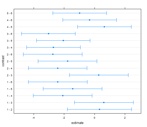
> # NB these give us the lsmeans AND the pairwise differences > # amongst lsmeans, using a Tukey approach (default) for the multiple comparison > # issue (which seems reasonable). We can specify other options, see examples > # For other linear combinations maybe it is most sensible to use > # Scheffé's test methods (see below) > # > lsmeans(lm1,pairwise~Diet) $lsmeans Diet lsmean SE df lower.CL upper.CL 1 4.609598 0.6828153 13 3.134465 6.084731 2 4.281027 0.6828153 13 2.805894 5.756160 3 4.000000 0.5767166 13 2.754080 5.245920 4 6.700000 0.5767166 13 5.454080 7.945920 5 6.050000 0.5767166 13 4.804080 7.295920 6 7.025000 0.5767166 13 5.779080 8.270920 Results are averaged over the levels of: Parity Confidence level used: 0.95 $contrasts contrast estimate SE df t.ratio p.value 1 - 2 0.3285714 0.9748290 13 0.337 0.9993 1 - 3 0.6095982 0.8937778 13 0.682 0.9809 1 - 4 -2.0904018 0.8937778 13 -2.339 0.2464 1 - 5 -1.4404018 0.8937778 13 -1.612 0.6057 1 - 6 -2.4154018 0.8937778 13 -2.702 0.1406 2 - 3 0.2810268 0.8937778 13 0.314 0.9995 2 - 4 -2.4189732 0.8937778 13 -2.706 0.1397 2 - 5 -1.7689732 0.8937778 13 -1.979 0.4024 2 - 6 -2.7439732 0.8937778 13 -3.070 0.0764 3 - 4 -2.7000000 0.8156004 13 -3.310 0.0505 3 - 5 -2.0500000 0.8156004 13 -2.513 0.1894 3 - 6 -3.0250000 0.8156004 13 -3.709 0.0251 4 - 5 0.6500000 0.8156004 13 0.797 0.9631 4 - 6 -0.3250000 0.8156004 13 -0.398 0.9984 5 - 6 -0.9750000 0.8156004 13 -1.195 0.8315 Results are averaged over the levels of: Parity P value adjustment: tukey method for comparing a family of 6 estimates > lsmeans(lm1,pairwise~Diet,adjust="Tukey") $lsmeans Diet lsmean SE df lower.CL upper.CL 1 4.609598 0.6828153 13 3.134465 6.084731 2 4.281027 0.6828153 13 2.805894 5.756160 3 4.000000 0.5767166 13 2.754080 5.245920 4 6.700000 0.5767166 13 5.454080 7.945920 5 6.050000 0.5767166 13 4.804080 7.295920 6 7.025000 0.5767166 13 5.779080 8.270920 Results are averaged over the levels of: Parity Confidence level used: 0.95 $contrasts contrast estimate SE df t.ratio p.value 1 - 2 0.3285714 0.9748290 13 0.337 0.9993 1 - 3 0.6095982 0.8937778 13 0.682 0.9809 1 - 4 -2.0904018 0.8937778 13 -2.339 0.2464 1 - 5 -1.4404018 0.8937778 13 -1.612 0.6057 1 - 6 -2.4154018 0.8937778 13 -2.702 0.1406 2 - 3 0.2810268 0.8937778 13 0.314 0.9995 2 - 4 -2.4189732 0.8937778 13 -2.706 0.1397 2 - 5 -1.7689732 0.8937778 13 -1.979 0.4024 2 - 6 -2.7439732 0.8937778 13 -3.070 0.0764 3 - 4 -2.7000000 0.8156004 13 -3.310 0.0505 3 - 5 -2.0500000 0.8156004 13 -2.513 0.1894 3 - 6 -3.0250000 0.8156004 13 -3.709 0.0251 4 - 5 0.6500000 0.8156004 13 0.797 0.9631 4 - 6 -0.3250000 0.8156004 13 -0.398 0.9984 5 - 6 -0.9750000 0.8156004 13 -1.195 0.8315 Results are averaged over the levels of: Parity P value adjustment: tukey method for comparing a family of 6 estimates > lsmeans(lm1,pairwise~Diet,adjust="Bonferroni") $lsmeans Diet lsmean SE df lower.CL upper.CL 1 4.609598 0.6828153 13 3.134465 6.084731 2 4.281027 0.6828153 13 2.805894 5.756160 3 4.000000 0.5767166 13 2.754080 5.245920 4 6.700000 0.5767166 13 5.454080 7.945920 5 6.050000 0.5767166 13 4.804080 7.295920 6 7.025000 0.5767166 13 5.779080 8.270920 Results are averaged over the levels of: Parity Confidence level used: 0.95 $contrasts contrast estimate SE df t.ratio p.value 1 - 2 0.3285714 0.9748290 13 0.337 1.0000 1 - 3 0.6095982 0.8937778 13 0.682 1.0000 1 - 4 -2.0904018 0.8937778 13 -2.339 0.5395 1 - 5 -1.4404018 0.8937778 13 -1.612 1.0000 1 - 6 -2.4154018 0.8937778 13 -2.702 0.2716 2 - 3 0.2810268 0.8937778 13 0.314 1.0000 2 - 4 -2.4189732 0.8937778 13 -2.706 0.2696 2 - 5 -1.7689732 0.8937778 13 -1.979 1.0000 2 - 6 -2.7439732 0.8937778 13 -3.070 0.1342 3 - 4 -2.7000000 0.8156004 13 -3.310 0.0845 3 - 5 -2.0500000 0.8156004 13 -2.513 0.3888 3 - 6 -3.0250000 0.8156004 13 -3.709 0.0394 4 - 5 0.6500000 0.8156004 13 0.797 1.0000 4 - 6 -0.3250000 0.8156004 13 -0.398 1.0000 5 - 6 -0.9750000 0.8156004 13 -1.195 1.0000 Results are averaged over the levels of: Parity P value adjustment: bonferroni method for 15 tests > lsmeans(lm1,pairwise~Diet,adjust="Scheffe") $lsmeans Diet lsmean SE df lower.CL upper.CL 1 4.609598 0.6828153 13 3.134465 6.084731 2 4.281027 0.6828153 13 2.805894 5.756160 3 4.000000 0.5767166 13 2.754080 5.245920 4 6.700000 0.5767166 13 5.454080 7.945920 5 6.050000 0.5767166 13 4.804080 7.295920 6 7.025000 0.5767166 13 5.779080 8.270920 Results are averaged over the levels of: Parity Confidence level used: 0.95 $contrasts contrast estimate SE df t.ratio p.value 1 - 2 0.3285714 0.9748290 13 0.337 0.9997 1 - 3 0.6095982 0.8937778 13 0.682 0.9918 1 - 4 -2.0904018 0.8937778 13 -2.339 0.4091 1 - 5 -1.4404018 0.8937778 13 -1.612 0.7574 1 - 6 -2.4154018 0.8937778 13 -2.702 0.2681 2 - 3 0.2810268 0.8937778 13 0.314 0.9998 2 - 4 -2.4189732 0.8937778 13 -2.706 0.2668 2 - 5 -1.7689732 0.8937778 13 -1.979 0.5794 2 - 6 -2.7439732 0.8937778 13 -3.070 0.1655 3 - 4 -2.7000000 0.8156004 13 -3.310 0.1181 3 - 5 -2.0500000 0.8156004 13 -2.513 0.3366 3 - 6 -3.0250000 0.8156004 13 -3.709 0.0657 4 - 5 0.6500000 0.8156004 13 0.797 0.9836 4 - 6 -0.3250000 0.8156004 13 -0.398 0.9994 5 - 6 -0.9750000 0.8156004 13 -1.195 0.9125 Results are averaged over the levels of: Parity P value adjustment: scheffe method with dimensionality 5 > lsmeans(lm1,pairwise~Parity) $lsmeans Parity lsmean SE df lower.CL upper.CL 1 4.266667 0.4708871 13 3.249377 5.283956 2 4.773065 0.5302150 13 3.627606 5.918525 3 6.987351 0.5302150 13 5.841891 8.132811 4 5.750000 0.4708871 13 4.732710 6.767290 Results are averaged over the levels of: Diet Confidence level used: 0.95 $contrasts contrast estimate SE df t.ratio p.value 1 - 2 -0.5063988 0.7091280 13 -0.714 0.8897 1 - 3 -2.7206845 0.7091280 13 -3.837 0.0097 1 - 4 -1.4833333 0.6659350 13 -2.227 0.1670 2 - 3 -2.2142857 0.7550993 13 -2.932 0.0502 2 - 4 -0.9769345 0.7091280 13 -1.378 0.5338 3 - 4 1.2373512 0.7091280 13 1.745 0.3413 Results are averaged over the levels of: Diet P value adjustment: tukey method for comparing a family of 4 estimates > lsmeans(lm1,pairwise~Diet,glhargs=list()) $lsmeans Diet lsmean SE df lower.CL upper.CL 1 4.609598 0.6828153 13 3.134465 6.084731 2 4.281027 0.6828153 13 2.805894 5.756160 3 4.000000 0.5767166 13 2.754080 5.245920 4 6.700000 0.5767166 13 5.454080 7.945920 5 6.050000 0.5767166 13 4.804080 7.295920 6 7.025000 0.5767166 13 5.779080 8.270920 Results are averaged over the levels of: Parity Confidence level used: 0.95 $contrasts contrast estimate SE df t.ratio p.value 1 - 2 0.3285714 0.9748290 13 0.337 0.9993 1 - 3 0.6095982 0.8937778 13 0.682 0.9809 1 - 4 -2.0904018 0.8937778 13 -2.339 0.2464 1 - 5 -1.4404018 0.8937778 13 -1.612 0.6057 1 - 6 -2.4154018 0.8937778 13 -2.702 0.1406 2 - 3 0.2810268 0.8937778 13 0.314 0.9995 2 - 4 -2.4189732 0.8937778 13 -2.706 0.1397 2 - 5 -1.7689732 0.8937778 13 -1.979 0.4024 2 - 6 -2.7439732 0.8937778 13 -3.070 0.0764 3 - 4 -2.7000000 0.8156004 13 -3.310 0.0505 3 - 5 -2.0500000 0.8156004 13 -2.513 0.1894 3 - 6 -3.0250000 0.8156004 13 -3.709 0.0251 4 - 5 0.6500000 0.8156004 13 0.797 0.9631 4 - 6 -0.3250000 0.8156004 13 -0.398 0.9984 5 - 6 -0.9750000 0.8156004 13 -1.195 0.8315 Results are averaged over the levels of: Parity P value adjustment: tukey method for comparing a family of 6 estimates > lsm2<-lsmeans(lm1,pairwise~Diet,glhargs=list()) > plot(lsm2[[2]]) > lsm2 $lsmeans Diet lsmean SE df lower.CL upper.CL 1 4.609598 0.6828153 13 3.134465 6.084731 2 4.281027 0.6828153 13 2.805894 5.756160 3 4.000000 0.5767166 13 2.754080 5.245920 4 6.700000 0.5767166 13 5.454080 7.945920 5 6.050000 0.5767166 13 4.804080 7.295920 6 7.025000 0.5767166 13 5.779080 8.270920 Results are averaged over the levels of: Parity Confidence level used: 0.95 $contrasts contrast estimate SE df t.ratio p.value 1 - 2 0.3285714 0.9748290 13 0.337 0.9993 1 - 3 0.6095982 0.8937778 13 0.682 0.9809 1 - 4 -2.0904018 0.8937778 13 -2.339 0.2464 1 - 5 -1.4404018 0.8937778 13 -1.612 0.6057 1 - 6 -2.4154018 0.8937778 13 -2.702 0.1406 2 - 3 0.2810268 0.8937778 13 0.314 0.9995 2 - 4 -2.4189732 0.8937778 13 -2.706 0.1397 2 - 5 -1.7689732 0.8937778 13 -1.979 0.4024 2 - 6 -2.7439732 0.8937778 13 -3.070 0.0764 3 - 4 -2.7000000 0.8156004 13 -3.310 0.0505 3 - 5 -2.0500000 0.8156004 13 -2.513 0.1894 3 - 6 -3.0250000 0.8156004 13 -3.709 0.0251 4 - 5 0.6500000 0.8156004 13 0.797 0.9631 4 - 6 -0.3250000 0.8156004 13 -0.398 0.9984 5 - 6 -0.9750000 0.8156004 13 -1.195 0.8315 Results are averaged over the levels of: Parity P value adjustment: tukey method for comparing a family of 6 estimates
and here is a graph of the pairwise differences amongst the diets:

